Upgrading PostgreSQL and PostGIS from 9.3 to 9.4

In this post, we will walk through steps of upgrading from PostgreSQL 9.3 to 9.4. It all happened because my PostGIS version had got corrupted.

When I executed the command to check for my PostGIS version, I got an error saying liblwgeom library could not be loaded

su - postgres -c "psql -c 'SELECT PostGIS_full_version()'"

gave the following error

ERROR:  could not load library "/usr/lib/postgresql/9.3/lib/postgis-2.1.so": liblwgeom-2.1.2.so: cannot open shared object file: No such file or directory

After much research and browsing through forums, I realized it was better to upgrade postgreSQL and PostGIS. I checked the postgres version with the following command to make sure I needed to do that.

I found a great post on stackexchange from someone who had posted their script. With minor changes the script was good. Here is the modified script in its entirety

I executed the following step by step to make sure I could see what was happening...

su - postgres -c "psql -c 'SELECT PostGIS_full_version()'"
su - postgres -c "psql --version"


# Be sure to save your config files.
sudo cp /etc/postgresql/9.3/main/postgresql.conf ~
sudo cp /etc/postgresql/9.3/main/pg_hba.conf ~

# Package repo (for apt-get). I have 14.04 LTS, so I selected trusty-pgdg. Please change to match your version
wget --quiet -O - https://www.postgresql.org/media/keys/ACCC4CF8.asc | sudo apt-key add -
sudo sh -c 'echo "deb http://apt.postgresql.org/pub/repos/apt/ trusty-pgdg main" >> /etc/apt/sources.list.d/postgresql.list'

# Also probably optional but I like to update sources and upgrade
sudo apt-get update
sudo apt-get upgrade

# Install postgres 9.4
sudo apt-get install postgresql-9.4 postgresql-server-dev-9.4 postgresql-contrib-9.4

# Get latest postgis for 9.4 (optional)
sudo apt-get install postgresql-9.4-postgis

# dump your data
sudo su postgres
cd ./data/dumps
/usr/lib/postgresql/9.4/bin/pg_dumpall > pre_upgrade_from_9.3_to_9.4.dump

# I got this error:
# pg_dump: [archiver (db)] query failed: ERROR:  could not load library "/usr/lib/postgresql/9.3/lib/postgis-2.1.so": 
# liblwgeom-2.1.2.so: cannot open shared object file: No such file or directory

#This is the elusive fix to the problem
sudo apt-get install liblwgeom-2.1.3

# Then repeated
sudo su postgres
cd ./data/dumps
/usr/lib/postgresql/9.4/bin/pg_dumpall > pre_upgrade_from_9.3_to_9.4.dump

# Make a data dir for Postgres 9.4
sudo mkdir -p /data/postgres/9.4/main
sudo chown -R postgres:postgres /data/postgres

# Change the 9.4 conf file's data dir to point to /data/postgres/9.4/main
sudo gedit /etc/postgresql/9.4/main/postgresql.conf

# Install 9.4 cluster
sudo /etc/init.d/postgresql stop

# May need to restart machine if could not stop both postgreSQL processes
sudo pg_dropcluster 9.4 main
sudo pg_createcluster -d /data/postgres/9.4/main 9.4 main

# start 9.4 explicitly
sudo /etc/init.d/postgresql start 9.4

# Restore: Make sure to use the 9.4 version of psql
psql -d postgres -p 5433 -f ~/data/dumps/pre_upgrade_from_9.3_to_9.4.dump

# Change port back to 5432 (optional) and the confs back to what they were! (reference previously copied files)
sudo gedit /etc/postgresql/9.4/main/postgresql.conf

# Changed local   all   all   peer -> local   all   all   md5
sudo gedit /etc/postgresql/9.4/main/pg_hba.conf

sudo service postgresql restart 9.4

# Verify your data was properly imported

# Drop old cluster
sudo pg_dropcluster --stop 9.3 main


# Analyze
sudo service postgresql start
psql
>\c your_database
> ANALYZE;

Now on starting I still got 2 postgres instances

We need to delete the old PostgreSQL version using commands below... 

#Delete previous postgres
sudo apt-get purge postgresql-9.3
sudo service postgresql restart 9.4

After the restart, it shows only one service starting..

Now, we can verify if PostGIS is correctly installed

su - postgres -c "psql -c 'SELECT PostGIS_full_version()'"

This shows the correct versions and everything should be fine. Finally to check the version of other extensions as well, we can use the following command

psql -c "SELECT name, default_version,installed_version FROM pg_available_extensions WHERE name LIKE 'postgis%'"

Looks like everything has got upgraded correctly.

Plotting R data on an Interactive Google map

In this post, we will see how to plot data on an interactive map using R. We will use Google maps as the base map. Here is the output

You can also switch to street view

Let's get started. Make sure you have installed the required libraries. The new library needed is googleVis which can be installed by launching R in sudo mode and entering the following command

install.packages("googleVis")
q()

First step is to download the data. This previous post shows how to obtain the spatial data used in this example from the NYC website. Now launch R in regular mode and enter the following code to create the map.

First we need to load the required libraries

# Load the needed libraries
library(sp)  # classes for spatial data
library(maptools)
library(rgeos) # and their dependencies
library(rgdal)
library(ggplot2)
library(ggmap)
library(scales)
library(gmodels)
library(googleVis)

Next we need to set the working directory where our scripts are located and declare a variable to folder where our data is located.

# Set default paths for data
setwd("~/Work/Transportation/NYC/scripts")
shpfilepath="../data/shpfiles"

Next we will read the shape files with data. We have two shape files from NYC. First contains only fatal accidents, and second contains injury accidents. We will later combine these files.

# Read injury and fatality statistics
ogrInfo(shpfilepath,"fatality_yearly")
ogrInfo(shpfilepath,"injury_yearly")
ftlty<-readOGR(shpfilepath, "fatality_yearly")
injry<-readOGR(shpfilepath, "injury_yearly")
names(ftlty); dim(ftlty)
names(injry); dim(injry)

Next we need to rename the column names across the two datasets so that they are identical. Following step shows us how to do that. We also will add a new variable that classifies the incident as an injury or a fatality incident.

#Classify severity and rename columns to be identical in fatalities and injury datasets
ftlty$Severity<-"Fatality"
names(ftlty)[names(ftlty)=="Fatalities"]<-"Total"
names(ftlty)[names(ftlty)=="PedFatalit"]<-"Ped"
names(ftlty)[names(ftlty)=="BikeFatali"]<-"Bike"
names(ftlty)[names(ftlty)=="MVOFatalit"]<-"MVO"
injry$Severity<-"Injury"
names(injry)[names(injry)=="Injuries"]<-"Total"
names(injry)[names(injry)=="PedInjurie"]<-"Ped"
names(injry)[names(injry)=="BikeInjuri"]<-"Bike"
names(injry)[names(injry)=="MVOInjurie"]<-"MVO"
names(injry);names(ftlty)

Now we can combine the two datasets to create one single dataset called acc.

#Combine datasets
acc<- rbind(ftlty, injry)
dim(acc);names(acc);head(acc)

We need to use the fortify command to make sure the coordinate information can be accessed by spatial functions.

#Now fortify the accident data
acc.f<-fortify(as.data.frame(acc))
dim(acc.f);names(acc.f);head(acc.f)

We only want to plot 2015 data. The following command shows us how to filter only 2015 records from the data.

#Subsetting only 2015 accident records
acc_2015<-acc.f[which(acc.f$YR==2015),] 

Now we are ready to plot this on the map. The gvisMap function expects a single field with latitude and longitude information in lat:long format, that is separated by a colon. We don't need more than 4 digit precision so we will round the lat long information and use the paste command to concatenate everything into a single string.

#Add a single column "LatLong" that is of the format lat:long for the accident location
acc_2015$LatLong<-paste(round(acc_2015$coords.x2,4),round(acc_2015$coords.x1,4),sep=":")

The gVisMap function also expects a data field which will be displayed as a map tip. We need to concatenate all available fields with html break symbol to create one single field that can pop up when we hover or click on the icon.

#Add a single column "Tip" for Accident descriptions separated by html breaks ("<br/>")
acc_2015$Tip<-paste("Type: ",acc_2015$Severity,"Total: ",acc_2015$Total,"Ped: ",acc_2015$Ped,"Bike: ",acc_2015$Bike,"MVO: ",acc_2015$MVO,sep="<br/>")
head(acc_2015)

Finally, we call the gVisMap function passing the dataset, name of concatenated lat long column, name of the Map tip column and set several defaults for the Google map. Calling the plot function launches an embedded http server and launches the default browser on your machine to display the generated html page.

#Plot 2015 accidents on Google
map1<-gvisMap(acc_2015, "LatLong", "Tip", 
              options=list(showTip=TRUE, showLine=F, enableScrollWheel=TRUE, 
                           mapType='roads', useMapTypeControl=TRUE, width=800,height=1024))
plot(map1)

That's it... We are done. Here is the output

Here is the complete source code

# Load the needed libraries
library(sp)  # classes for spatial data
library(maptools)
library(rgeos) # and their dependencies
library(rgdal)
library(ggplot2)
library(ggmap)
library(scales)
library(gmodels)
library(googleVis)

# Set default paths for data
setwd("~/Work/Transportation/NYC/scripts")
shpfilepath="../data/shpfiles"

# Read injury and fatality statistics
ogrInfo(shpfilepath,"fatality_yearly")
ogrInfo(shpfilepath,"injury_yearly")
ftlty<-readOGR(shpfilepath, "fatality_yearly")
injry<-readOGR(shpfilepath, "injury_yearly")
names(ftlty); dim(ftlty)
names(injry); dim(injry)

#Classify severity and rename columns to be identical in fatalities and injury datasets
ftlty$Severity<-"Fatality"
names(ftlty)[names(ftlty)=="Fatalities"]<-"Total"
names(ftlty)[names(ftlty)=="PedFatalit"]<-"Ped"
names(ftlty)[names(ftlty)=="BikeFatali"]<-"Bike"
names(ftlty)[names(ftlty)=="MVOFatalit"]<-"MVO"
injry$Severity<-"Injury"
names(injry)[names(injry)=="Injuries"]<-"Total"
names(injry)[names(injry)=="PedInjurie"]<-"Ped"
names(injry)[names(injry)=="BikeInjuri"]<-"Bike"
names(injry)[names(injry)=="MVOInjurie"]<-"MVO"
names(injry);names(ftlty)

#Combine datasets
acc<- rbind(ftlty, injry)
dim(acc);names(acc);head(acc)

#Now fortify the accident data
acc.f<-fortify(as.data.frame(acc))
dim(acc.f);names(acc.f);head(acc.f)

#Subsetting only 2015 accident records
acc_2015<-acc.f[which(acc.f$YR==2015),] 

#Add a single column "LatLong" that is of the format lat:long for the accident location
acc_2015$LatLong<-paste(round(acc_2015$coords.x2,4),round(acc_2015$coords.x1,4),sep=":")

#Add a single column "Tip" for Accident descriptions separated by html breaks ("<br/>")
acc_2015$Tip<-paste("Type: ",acc_2015$Severity,"Total: ",acc_2015$Total,"Ped: ",acc_2015$Ped,"Bike: ",acc_2015$Bike,"MVO: ",acc_2015$MVO,sep="<br/>")
head(acc_2015)

#Plot 2015 accidents on Google
map1<-gvisMap(acc_2015, "LatLong", "Tip", 
              options=list(showTip=TRUE, showLine=F, enableScrollWheel=TRUE, 
                           mapType='roads', useMapTypeControl=TRUE, width=800,height=1024))
plot(map1)

Steps for installing dismo in R

Steps for installing dismo in your R distribution are fairly straight forward.

First login to R using sudo, so your package can be installed to the shared repository

sudo R

Next, enter the following command in R prompt

install.packages("dismo")

By default, R prompts for https mirrors. For some reason, https mirrors gave me errors. For this reason select the option for HTTP mirrors at the bottom of the list, as shown below.

Next, choose your preferred mirror from the list of http mirrors, as shown below

Click OK to install. R will download the packages and install as neccessary.

Once the installation, has finished load the library using the following command and we are good to go.

library(dismo)

That's it...

Performing Spatial Overlay and CrossTab in R

In this post, we will look at spatial overlay in R using a simple example.

Here are the results we will produce



In previous posts, we had seen how to render multiple layers in R using ggplot2. This post will use the same dataset but for a different purpose.

First step is to download the data. This previous post shows how to obtain the spatial data used in this example from the NYC website.

Launch R in a terminal and load the required libraries. I have posted in previous posts on how to install these libraries. This post describes rgdal and associated packages' installation. This post describes gmodels package installation.

# Load required libraries
library(rgdal)
library(ggplot2)
library(ggmap)
library(rgeos)
library(maptools)
library(scales)
library(gmodels)

Next we set the default paths for the data. Please modify this accordingly for your environment

# Set default paths for data
setwd("~/Work/Transportation/NYC/scripts")
shpfilepath="../data/shpfiles"

Now we can read the shapefiles into our workspace memory for analysis

# Read injury and fatality statistics
ogrInfo(shpfilepath,"fatality_yearly")
ogrInfo(shpfilepath,"injury_yearly")
ftlty_yr<-readOGR(shpfilepath, "fatality_yearly")
injry_yr<-readOGR(shpfilepath, "injury_yearly")
names(ftlty_yr); dim(ftlty_yr)
names(injry_yr); dim(injry_yr)

Successful reading will show the following results.

As we can see from the names description, the data does not have any spatial information attached. We need to use the fortify command to attach the spatial coordinates to the data we have.

# Add the spatial data to the data frame
ftlty.f <-fortify(as.data.frame(ftlty_yr))
names(ftlty.f);dim(ftlty.f)

Using the fortify command attaches the spatial data to our previous structure as can be seen in the console output.

Next we look at the New York City Borough boundaries that we need to use.

#Load boroughs data
ogrInfo(shpfilepath,"nybbwi")
bbnd <- readOGR(shpfilepath,"nybbwi")

As we can see the borough layer has lambert conformal conic coordinate reference system, which means that the fatality data and boundaries will not coincide. We will use the spTransform function to transform the boundaries from lambert conformal to lat long.

#Transform the coordinates from Lambert Conformal to Lat Long
CRS.latlong<-CRS("+proj=longlat +datum=WGS84 +no_defs")
bbnd<-spTransform(bbnd, CRS.latlong)
summary(bbnd)

As we can see the data has been transformed. We need to also fortify the boundary data to attach the spatial information.

# Add the spatial data back to the boundary data.frame
bbnd.f <-fortify(bbnd, region="BoroCode")
names(bbnd.f);head(bbnd.f);dim(bbnd.f)

Now that we have the geometric information attached, the number of rows increases to include each part of each geometric record. We need to re-attach the attribute information for each geometric part, using the merge command.

# Combine the geometry and data back together using common keys
bbnd.f<-merge(bbnd.f,bbnd@data, by.x="id", by.y="BoroCode")
names(bbnd.f);head(bbnd.f);dim(bbnd.f)

As we can see the information has been attached, and now we have 7+3 = 10 columns of data for the polygon dataset. Now the overlay. We will attach each fatality record the borough it falls in. The over() function allows that. We will also take this information and add it to two new variables in the ftlty.f data frame. R will take care of altering the structure of the table to accommodate the new data points.

#Code each record in fatality with the borough it falls under and add to new variable
ftlty.f$BoroCode <-as.data.frame(over(ftlty_yr, bbnd))$BoroCode
ftlty.f$BoroName <-as.data.frame(over(ftlty_yr, bbnd))$BoroName
names(ftlty.f);head(ftlty.f);dim(ftlty.f)

As we can see new information has been attached. Each accident record has been coded with the borough it falls in. We can infact use the following code to plot it to a map.

#Plot accidents coded by the borough they fall in
fx<-ftlty.f$coords.x1
fy<-ftlty.f$coords.x2
Map <- ggplot(data=ftlty.f, aes(fx,fy,colour=factor(BoroCode)))
Map <- Map + layer(geom="point")
Map

The following map is generated

Next we will use the CrossTable function to look at number of accidents that involved one or more fatalities

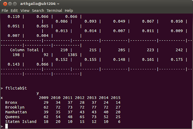
We can instead also build a table to summarize fatalities by borough and year.

#Build a cross table for Borough name and Year with count of fatal incidents
ftlctab<-CrossTable(ftlty.f$BoroName,ftlty.f$YR,expected=FALSE)
ftlctab$t

We can also build a cross table to look at number of fatalities using the xtabs function.

#Build a cross table for Borough name and Year with fatalities
ftlctab2<-xtabs(ftlty.f$Fatalities ~  ftlty.f$BoroName+ftlty.f$YR,ftlty.f)
ftlctab2

We can actually compare the results in the output above to see the differences.

We can also plot the above in barplots using the barplot command.

#Plot this on a barplot to see the trends for Incidents with fatalities
barplot(ftlctab$t 
 ,col=c("red","orange","yellow","green","blue", "darkblue","grey")
 ,names.arg=levels(ftlty.f$YR)
 ,legend=rownames(ftlty.f$BoroName)
)

Now we could also plot the sum of fatalities instead of fatal incidents by using the ftlctab2 variable instead.

#Plot this on a barplot to see the trends for Fatalities
barplot(ftlctab2
 ,col=c("red","orange","yellow","green","blue", "darkblue","grey")
 ,names.arg=levels(ftlty.f$YR)
 ,legend=levels(ftlty.f$BoroName)
)

That's it. Here is the complete source code

# Load required libraries
library(rgdal)
library(ggplot2)
library(ggmap)
library(rgeos)
library(maptools)
library(scales)
library(gmodels)

# Set default paths for data
setwd("~/Work/Transportation/NYC/scripts")
shpfilepath="../data/shpfiles"

# Read injury and fatality statistics
ogrInfo(shpfilepath,"fatality_yearly")
ogrInfo(shpfilepath,"injury_yearly")
ftlty_yr<-readOGR(shpfilepath, "fatality_yearly")
injry_yr<-readOGR(shpfilepath, "injury_yearly")
names(ftlty_yr); dim(ftlty_yr)
names(injry_yr); dim(injry_yr)

# Add the spatial data to the data frame
ftlty.f <-fortify(as.data.frame(ftlty_yr))
names(ftlty.f);dim(ftlty.f)

#Load boroughs data
ogrInfo(shpfilepath,"nybbwi")
bbnd <- readOGR(shpfilepath,"nybbwi")

#Transform the coordinates from Lambert Conformal to Lat Long
CRS.latlong<-CRS("+proj=longlat +datum=WGS84 +no_defs")
bbnd<-spTransform(bbnd, CRS.latlong)

# Add the spatial data back to the boundary data.frame
bbnd.f <-fortify(bbnd, region="BoroCode")
names(bbnd.f);head(bbnd.f);dim(bbnd.f)

# Combine the geometry and data back together using common keys
bbnd.f<-merge(bbnd.f,bbnd@data, by.x="id", by.y="BoroCode")
names(bbnd.f);head(bbnd.f);dim(bbnd.f)

#Code each record in fatality with the borough it falls under and add to new variable
ftlty.f$BoroCode <-as.data.frame(over(ftlty_yr, bbnd))$BoroCode
ftlty.f$BoroName <-as.data.frame(over(ftlty_yr, bbnd))$BoroName
names(ftlty.f);head(ftlty.f);dim(ftlty.f)

#Plot accidents coded by the borough they fall in
fx<-ftlty.f$coords.x1
fy<-ftlty.f$coords.x2
Map <- ggplot(data=ftlty.f, aes(fx,fy,colour=factor(BoroCode)))
Map <- Map + layer(geom="point")
Map

#Build a cross table for Borough name and Year with count of fatal incidents
ftlctab<-CrossTable(ftlty.f$BoroName,ftlty.f$YR,expected=FALSE)
ftlctab$t

#Build a cross table for Borough name and Year with fatalities
ftlctab2<-xtabs(ftlty.f$Fatalities ~  ftlty.f$BoroName+ftlty.f$YR,ftlty.f)
ftlctab2

#Plot this on a barplot to see the trends for Incidents with fatalities
barplot(ftlctab$t 
 ,col=c("red","orange","yellow","green","blue", "darkblue","grey")
 ,names.arg=levels(ftlty.f$YR)
 ,legend=rownames(ftlty.f$BoroName)
)

#Plot this on a barplot to see the trends for Fatalities
barplot(ftlctab2
 ,col=c("red","orange","yellow","green","blue", "darkblue","grey")
 ,names.arg=levels(ftlty.f$YR)
 ,legend=levels(ftlty.f$BoroName)
)

Installing gmodels library in R

Steps for installing gmodels in your R distribution are fairly straight forward.

First login to R using sudo, so your package can be installed to the shared repository

sudo R

Next, enter the following command in R prompt

install.packages("gmodels")

By default, R prompts for https mirrors. For some reason, https mirrors gave me errors. For this reason select the option for HTTP mirrors at the bottom of the list, as shown below.

Next, choose your preferred mirror from the list of http mirrors, as shown below

Click OK to install. R will download the packages and install as neccessary.

Once the installation, has finished load the library using the following command and we are good to go.

library(gmodels)

That's it...

Building a multi-layer map in R using ggplot2 and spatial data

In this post, we will render spatial point and polygon data on the same map (as separate layers). The finished sample is the following:

This exercise involves using several libraries from R, as well as transforming data from one coordinate system to another. Here are the prerequisites

1. Install required spatial libraries into R: Please refer to this post, on how to do so.
2. Download spatial data for NYC pertaining to safety: Please refer to this post on how to do so.

So let's get started.

First step is to load all the libraries

# Load required libraries
library(rgdal)
library(ggplot2)
library(ggmap)
library(rgeos)
library(maptools)
library(scales)

Each of the above have a specific function in the process. Next step is to set the working directory for the data files. We use the setwd command for that and I have also set a variable for setting the shape file path.

# Set default paths for data
setwd("~/Work/Transportation/NYC/scripts")
shpfilepath="../data/shpfiles"

Next we read the shape files that contain annual fatality and injury data as well as data on borough boundaries for New York Let's start with the injury and fatality data. ogrInfo command provides high level summary of the data in each shape file.

# Read injury and fatality statistics
ogrInfo(shpfilepath,"fatality_yearly")
ogrInfo(shpfilepath,"injury_yearly")

Next, we read the shape file data into R and assign it to an R object variable.

ftlty_yr<-readOGR(shpfilepath, "fatality_yearly")
injry_yr<-readOGR(shpfilepath, "injury_yearly")
names(ftlty_yr); dim(ftlty_yr)
names(injry_yr); dim(injry_yr)

At this point the geometric data is not bound to the data frame, as we can see.

Also, lets create our first graph with ggplot. We read the data frame from the fatalities data. As we can see there is no geometry for us to plot at this point, so we will simply plot Fatalities against the year. GGPlot2 library distinguishes between data, aesthetics, from the graph. In the first example, we simply add the data to the base layer and ask ggplot to render it as a point.

# Extract the data frame and use ggplot
ftldata<-ftlty_yr@data
names(ftldata)
p<-ggplot(ftlty_yr@data, aes(Fatalities, YR))
p + geom_point()
p

This is the graph that was plotted...

This is our first attempt at understanding ggplot, but not what we wanted. The problem is that when we read the shapefile, the spatial data was not brought along.

We need to use the fortify command to add the spatial data. In the following steps, we can see how to do that. Once we fortify the data, we can extract the x and y coordinates as well.

ftlty.f <-fortify(as.data.frame(ftlty_yr))
names(ftlty.f);dim(ftlty.f)
fx<-ftlty.f$coords.x1
fy<-ftlty.f$coords.x2

Now, since we have the x and y, we can plot this data using ggplot

# Plotting the data using ggplot
Map <- ggplot(data=ftlty.f, aes(fx,fy,colour=factor(Fatalities)))
Map <- Map + layer(geom="point")
Map

Here is the plot output

Next step is to read the boroughs data. We use the familiar ogrInfo and readOGR functions to read the shapefile data into R

#Load boroughs data
ogrInfo(shpfilepath,"nybbwi")
bbnd <- readOGR(shpfilepath,"nybbwi")

The Boroughs data is in a different coordinate system than the accident data. While the accident data is in latitude longitude, the borough data is in Lambert conformal conic coordinate system. If we want to have the two map layers sit on top of one another, we need to have them in the same coordinate system. We use the spTransform function to transform the borough boundaries to latlong, as shown below...

#Transform the coordinates from Lambert Conformal to Lat Long
CRS.latlong<-CRS("+proj=longlat +datum=WGS84 +no_defs")
bbnd<-spTransform(bbnd, CRS.latlong)

In this case, again the spatial data and non-spatial data is not together. We need one dataset with both, so we need to fortify and merge the spatial and non-spatial datasets.

# Add the spatial data back to the boundary data.frame
bbnd.f <-fortify(bbnd, region="BoroCode")
names(bbnd.f);fix(bbnd.f);dim(bbnd.f)

# Combine the geometry and data back together using common keys
bbnd.f<-merge(bbnd.f,bbnd@data, by.x="id", by.y="BoroCode")
names(bbnd.f);dim(bbnd.f)

As we can see in the following window, using fortify alone brought in the 7 geometric attributes and merge brought the total to 10 attributes with attributes from the data frame. So, we need both fortify and merge commands to bring in the geometry and associated non-spatial attributes such as area and length together.

Next step is to build the map one layer at a time.

# Plot a map of the boroughs and accidents
baes <-aes(x=long, y=lat, group = group ,alpha=1/50,fill=id) # Aesthetics for Boroughs
bblyr <-geom_polygon(data=bbnd.f, baes) # Polygon layer for Bouroughs
faes <-aes(x=fx, y=fy, colour=factor(Fatalities)) # Aesthetics for Fatalities
flyr <-geom_point(data=ftlty.f,faes) # Point layer for Fatalities
Map <- ggplot() # Initialize the map
Map <-Map + bblyr # Add the boroughs layer
Map <-Map + flyr # Add the Fatalities layer
Map <- Map + labs(x = "Longitude", y = "Latitude", fill = "NYC Boroughs") # Add the labels
Map <- Map + ggtitle("NYC Boroughs with Accidents")
Map # Display the Map

Here is the console output.

Here is the map

That's it... For those who are interested, here is the complete source listing..

# Load required libraries
library(rgdal)
library(ggplot2)
library(ggmap)
library(rgeos)
library(maptools)
library(scales)

# Set default paths for data
setwd("~/Work/Transportation/NYC/scripts")
shpfilepath="../data/shpfiles"

# Read injury and fatality statistics
ogrInfo(shpfilepath,"fatality_yearly")
ogrInfo(shpfilepath,"injury_yearly")
ftlty_yr<-readOGR(shpfilepath, "fatality_yearly")
injry_yr<-readOGR(shpfilepath, "injury_yearly")
names(ftlty_yr); dim(ftlty_yr)
names(injry_yr); dim(injry_yr)

# Extract the data frame and use ggplot
ftldata<-ftlty_yr@data
names(ftldata)
p<-ggplot(ftlty_yr@data, aes(Fatalities, YR))
p + geom_point()
p

# Add the spatial data to the data frame
ftlty.f <-fortify(as.data.frame(ftlty_yr))
names(ftlty.f);dim(ftlty.f)
fx<-ftlty.f$coords.x1
fy<-ftlty.f$coords.x2

# Plotting the data using qplot
qplot(fx,fy,data=ftlty.f)
qplot(fx,fy,data=ftlty.f,colour=factor(Fatalities))
qplot(fx,fy, data=ftlty.f,colour=factor(Fatalities), facets= . ~ YR) + geom_point()

# Plotting the data using ggplot
Map <- ggplot(data=ftlty.f, aes(fx,fy,colour=factor(Fatalities)))
Map <- Map + layer(geom="point")
Map
 
#Load boroughs data
ogrInfo(shpfilepath,"nybbwi")
bbnd <- readOGR(shpfilepath,"nybbwi")

#Transform the coordinates from Lambert Conformal to Lat Long
CRS.latlong<-CRS("+proj=longlat +datum=WGS84 +no_defs")
bbnd<-spTransform(bbnd, CRS.latlong)

#Examine the data
bbndata <-bbnd@data
names(bbndata);fix(bbndata);dim(bbndata)

# Add the spatial data back to the boundary data.frame
bbnd.f <-fortify(bbnd, region="BoroCode")
names(bbnd.f);fix(bbnd.f);dim(bbnd.f)

# Combine the geometry and data back together using common keys
bbnd.f<-merge(bbnd.f,bbnd@data, by.x="id", by.y="BoroCode")
names(bbnd.f);dim(bbnd.f)

# Plot a map of the boroughs and accidents
baes<-aes(x=long, y=lat, group = group ,alpha=1/50,fill=id) # Aesthetics for Boroughs
bblyr<-geom_polygon(data=bbnd.f, baes) # Polygon layer for Bouroughs
faes<-aes(x=fx, y=fy, colour=factor(Fatalities)) # Aesthetics for Fatalities
flyr<-geom_point(data=ftlty.f,faes) # Point layer for Fatalities
Map <- ggplot() # Initialize the map
Map<-Map + bblyr # Add the boroughs layer
Map<-Map + flyr # Add the Fatalities layer
Map <- Map + labs(x = "Longitude", y = "Latitude", fill = "NYC Boroughs") # Add the labels
Map <- Map + ggtitle("NYC Boroughs with Accidents")
Map # Display the Map