Download and Install SUMO - Simulation of Urban MObility on Ubuntu

SUMO is an open source, microscopic and continuous road traffic simulation package designed to handle large road networks. The advantage is that it is open source. In this post, we will follow the steps to install SUMO on Ubuntu. The version we will install is Version 0.18.

The SUMO site is at the following location:

http://sumo-sim.org/

The downloads link provides the links to download and install the software.

We will install a pre-compiled binary to get started. To install the software on Ubuntu, we need to add the repository to the apt package using the following command.

$ sudo add-apt-repository ppa:sumo/stable

Entering gives several prompts for entering the password and confirming the installation.

Next, we need to install the sumo, sumo-tools and sumo-doc packages on our machine.

$ sudo apt-get install sumo sumo-tools sumo-doc

Entering the command downloads the files and prompts to start installation on the machine.

After clicking yes, SUMO is installed on the machine.

To check, open a new terminal window or within the same window, type the following command, and we can see the results from the program.

$ sumo --help

There we go, we have installed SUMO on our machine.

Happy simulating

Setting the schema (search_path) in psql using command line options

The need to set schema using command line options

I was looking at ways to set the search_path in psql using command line options. The reason being that I had a bunch of auto-generated sql scripts that I wanted to run for a specific schema in Postgresql. Turns out that there is no out of the box option to set the schema from command line options. However, it is fairly straightforward to add the option.

Verifying the default schema

By default, when a user logs into psql, the search_path includes the public and $user schema. This can be verified by entering the show search_path command on the psql terminal as shown below.

=> show search_path;

To change the default schema from the psql command line, the first step is to edit the .psqlrc file on your machine.

Editing the ~/.psqlrc file

Postgresql's psql file allows users to extend the behaviour of the psql tool. Open a terminal window and type in the following commands.

$ sudo gedit ~/.psqlrc

This will open the existing (or new) ~./psqlrc file on your machine for editing.

Add the following line to the file.

SET search_path TO :schema;

This exposes search_path as a variable that can be set from the command line. Now, specifying a schema as a parameter sets the schema(search_path) to the specified value, as shown below....

In the following statement, nystaging is the name of the schema I want to set the value to.

$ psql -U nydot -d nywarehouse -v schema=nystaging

This changes the default schema to nystaging. This can be verified again by entering the show search_path command, as shown below....

=> show search_path;

To revert to the default path, you can specify the default path as a command line parameter, or comment the line in ~./psqlrc file.

That's it.

Starting a Remote Session from one Ubuntu machine on another Ubuntu machine

In this article, we look at ways to start a remote session from one Ubuntu machine on another. First to clarify, starting a remote session is not the same as Desktop sharing with tools like VNC.

What I really wanted was to let the remote machine operate using display settings of my client machine. Reason was, on my primary machines at my home, I have a dual display with 23 and 24 inch monitors, one of which is rotated by 90 degrees. Trying to access this over VNC meant that my local view consisted of this extended desktop made up of display real estate that was impossible to manipulate over my client machine that was a laptop.

This requires two steps

1. Step 1: Connect to the machine using secure shell
2. Step 2: Launch a remote gnome session

Here are the steps.

Step 1: Connect to the machine using a secure shell

The first step was to open a terminal windows and start a sescure shell session.

$ ssh -X user@host_machine

For example, in my case that works out to the following:

$ ssh -X arthgallo@192.168.0.XX

It may show a prompt similar to following (I have blanked out my ECDSA key on purpose).

Say yes to continue.

You will have to enter your password to continue.

This will start the remote X session.

Step 2: Launch a remote gnome session

Next launch a gnome session using the following command.

$gnome-session –session=gnome-classic

The new gnome session is launched as part of the primary desktop, and we can see the remote machine's desktop on our machine.

That's it, we are done.

Creating the Time Dimension table in Pentaho Data Integration (Kettle)

In my previous post, we had seen how to create the Date Dimension table using Pentaho Data Integration (Kettle). In this post, we will see how to create a Time dimension in Kettle.

It is recommended that Time dimension be a separate dimension from the Date. In that spirit, I created the following transformation in Kettle. It contains the following 10 steps.

1. Launch Kettle

2. Generate Rows for processing and setup variables

3. Convert Date to Epoch Time

4. Create sequence for incrementing time in milliseconds

5. Create sequence for incrementing identifier

6. Increment time and identifier with newly created sequences

7. Convert time in milliseconds back to Date

8. Output contents to a text file

9. Extract time out of the incremented date

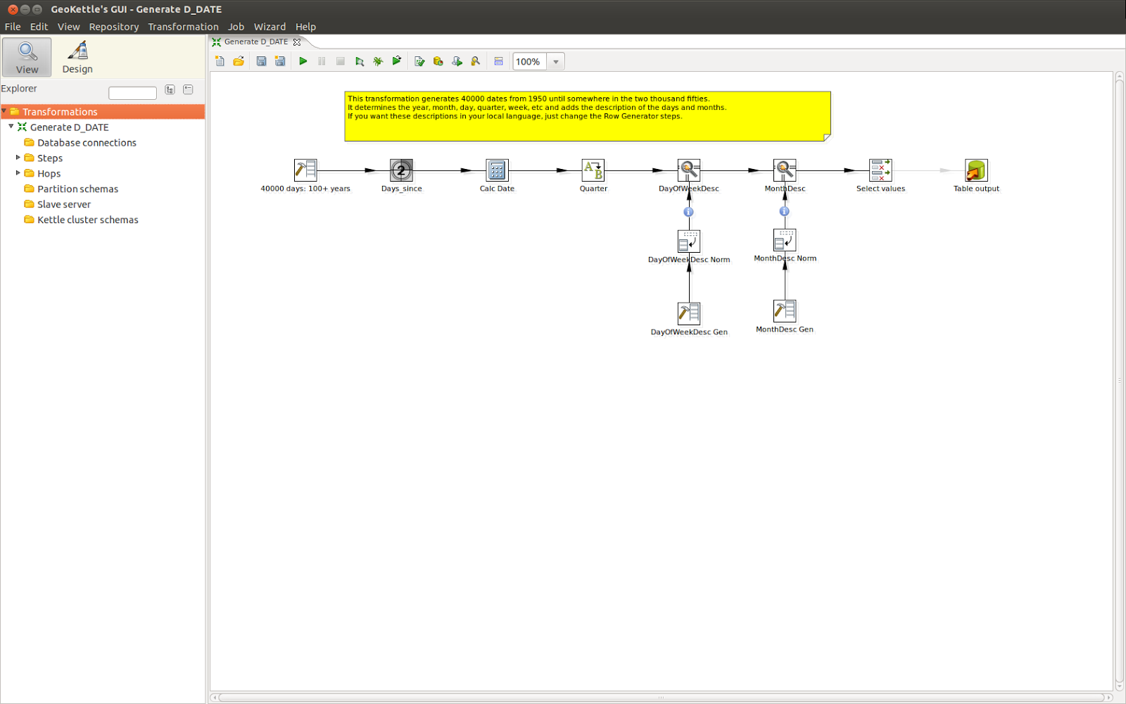
Step 1: Launch Kettle

Launch Pentaho Data Integration (Kettle or GeoKettle) on your local machine. Create a new transformation by clicking on File > New Transformation.

Step 2: Generate Rows for processing and setup variables

Make sure you are in design mode. Expand the Input section on Steps menu on the side and navigate to Generate Rows step.

Drag the Generate Rows step across to the work area as shown below, and drop it in the work area.

Right click on the Generate Rows step and enter the following information

1. Step Name: Generate Rows
2. Limit : 1440

In the fields column, add the following field

1. Name: START_TIME
2. Type: Integer
3. Format: ####
4. Value: 0000

Click on the row to add a second field. Add the following parameters for this field

1. Name: REAL_TIME
2. Type: Date
3. Format: yyyy/MM/dd HH:mm:ss
4. Value: 1970/01/01 00:00:00

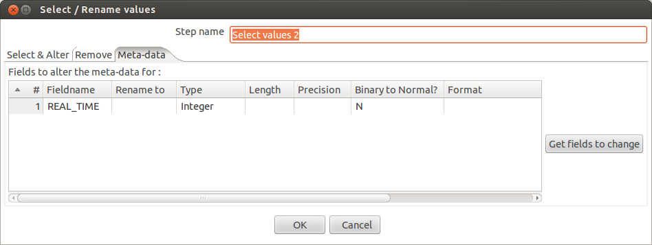
Step 3: Convert Date to Epoch Time

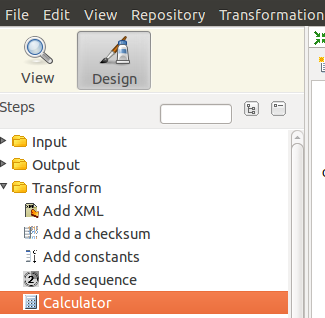
Next add “Select Values” from the Transform section of the Design tab. Select Values control allows us to change and modify the datatype of any variable in the flow. After dropping the step in the workspace, connect it to the preceding step using a hop as shown in the adjacent figure.

Now Edit the step to enter the following configuration information to convert Real time to an Integer. Doing so, converts the time to its Epoch time in milliseconds. To do so, we enter the following information.

1. Fieldname: REAL_TIME
2. Type: Integer

Step 4: Create sequence for incrementing time in milliseconds

Next we add a Sequence to our flow, and connect it to the preceding step as shown in the screenshots below. The sequence will increment our time in milliseconds derived in the previous step, by one minute intervals.

Edit the step in the transformation to enter the following information.

1. Step name: Millisecond Sequence
2. Name of value: MS_Increment
3. Use counter to calculate sequence:
4. Start at value: 0
5. Increment by: 60000
6. Maximum value: 86400000

Click OK to continue.

Step 5: Create sequence for incrementing identifier

Now add another sequence to the transformation as shown below and connect it to the preceding hop as shown below.

We can enter the following configuration for the newly added sequence.

1. Step name: Time_Since
2. Name of value: Time_Since
3. Use counter to calculate sequence:
4. Start at value: 0
5. Increment by: 1
6. Maximum value: 1440

Step 6: Increment time and identifier with newly created sequences

Next, we need to add a calculator to the flow.

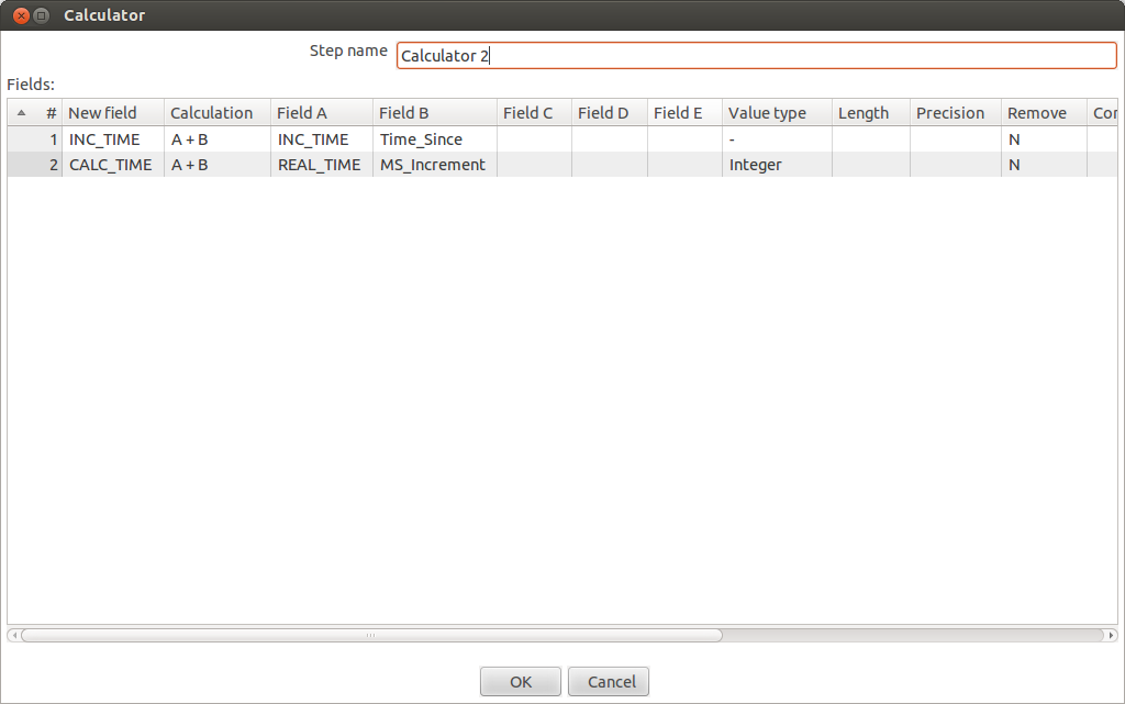
We need to configure the calculator by adding two calculations. First calculation adds the numeric sequence to our identifier, and second sequence adds Millisecond increments to our time.

For the first field, enter the following details.

New field: INC_TIME
Calculation: A+B

Field A: INC_TIME

Field B: Time_Since

Remove: N

For the next field, add the following parameters.

New field: CALC_TIME

Calculation: A+B

Field A: REAL_TIME

Field B: MS_Increment

Value type: Integer

Remove: N

Here is how the dialog box looks on my screen.

Click OK to continue.

Step 7: Convert time in milliseconds back to Date

Next step is to convert the calculated time from integer back to Date. To do this, we add another Select Values step to our transformation.

Make the following configuration changes in the newly added step.

Fieldname: CALC_TIME

Type: Date

Binary to Normal?: N

Format: yyyy/MM/dd HH:mm:ss

Click OK to continue

Step 8: Output contents to a text file

The final step is to output the contents to a text file

For this we add a “File Text Output” step to our transformation.

The Text File Output step, as the name suggests outputs the results to a text file.

Edit the “Text File Ouput” step, and make the following changes.

On the File tab, set the name of the output file. I have set it to simply “log” and the Extension to txt. This will create a file called log.txt in the output folder.

Step 9: Extract time out of the incremented date

Before clicking OK, switch to the Fields tab, and make the following entries.

Retain the following two fields.

1. Field 1 details are as follows

• Name: Time_Since
• Type: Integer
• Precision: 0

2. Field 2 details are as follows

• Name: CALC_TIME
• Type: Date
• Format: HH:mm:ss

The following screenshot shows these changes as on my screen.

Click Ok. 

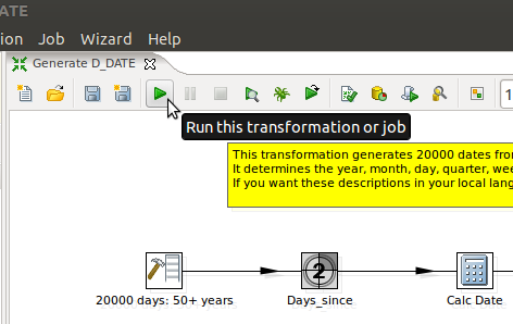
Step 10: Save and Test the Transformation

Save the transformation using the floppy icon on toolbar or File > Save on drop down menu.

Now, we need to run it using the Launch button.

Clicking this button launches the following screen.

Click the Launch button and the transformation starts executing.

The Execution Results window shows the results in a bottom pane.

Opening the log file, we can see the following results.

That's it, we are done.

Creating the Date Dimension using Kettle

Creating the Date dimension table is perhaps the most important common step to all dimensional modeling projects. According to Ralph Kimball – the author of The Data Warehousing Toolkit


“Data warehouses always need an explicit date dimension table. There are many date attributes not supported by the SQL Date function, including fiscal periods, seasons, holidays, and weekends. Rather than attempting to determine these nonstandard calendar calculations in a query, we should look them up in a date dimension table.”


The first step is to launch Kettle from the desktop. I have GeoKettle installed on my machine, which, for those who don't know, is simply a spatially enabled version of Pentaho's Open source ETL platform (Kettle). If you don't have GeoKettle installed, my previous post shows the steps to download and install it on your local machine.

Using the sample Transformation as the starting point.

GeoKettle ships with some sample transformations that allow creation of Date dimensions. We can start with these and augment them based on our needs. The first two dimensions that are needed are Date and Time. According to best practices, Date and Time should be modeled as separate dimensions

Launching GeoKettle

If you have GeoKettle installed, launch it from the Applications menu on your machine.

Once GeoKettle is launched, go to the samples folder under GeoKettle/samples and open the file “General – Populate date dimension.ktr”

The following transformation is loaded on the screen.

Save the file to your local directory for review and possible modification. I saved the transformation with the GenerateDateDimension.ktr under my local work folder.

The default transformation generates dates from 1950 all the way to 2050. I only needed 50 odd years of dates for my purposes, so I needed to modify the start date. Right click and Edit the first step on the transformation to view dialog box for "Generate Rows."

In the dialog box that opens, we can see the default values as follows:

Now lets modify the default values as follows.

Step name: 20000 days: 50+ years

Limit: 20000

Fields > Value: 19900101

Next thing we need to do is to update the Table output parameters to our selected database schema. Right click on the "Table Output" step as shown in the screenshot below.

Define the database connection, by clicking on the "New" button next to the Connection field on the open dialog box.

Select the schema and table name. In my case, it was nydot and dim_date.

Click OK when done. 

The last step is to enable the hop, by right clicking on the arrow connecting to the last step and clicking on “Enable Hop” as shown in the picture below.

Next step is to run the transformation and test to make sure it works correctly. For this we click on the play button on the top menu, as shown in the picture below.

Clicking the button brings up the following dialog box.

Now, click on the Launch button to start the transformation. Once the transformation has executed, we can see the following metrics displayed on the screen.

Open pgAdmin tool to view the data by navigating to the schema and the date_dim table that was just created.

Also, now right clicking and viewing data

.... shows that the table is populated correctly.

We have just seen how to populate a basic Date Dimension table using Kettle open source ETL tool.