Here are the results we will produce
In previous posts, we had seen how to render multiple layers in R using ggplot2. This post will use the same dataset but for a different purpose.
First step is to download the data. This previous post shows how to obtain the spatial data used in this example from the NYC website.
Launch R in a terminal and load the required libraries. I have posted in previous posts on how to install these libraries. This post describes rgdal and associated packages' installation. This post describes gmodels package installation.
# Load required libraries
library(rgdal)
library(ggplot2)
library(ggmap)
library(rgeos)
library(maptools)
library(scales)
library(gmodels)
Next we set the default paths for the data. Please modify this accordingly for your environment
# Set default paths for data
setwd("~/Work/Transportation/NYC/scripts")
shpfilepath="../data/shpfiles"
Now we can read the shapefiles into our workspace memory for analysis
# Read injury and fatality statistics
ogrInfo(shpfilepath,"fatality_yearly")
ogrInfo(shpfilepath,"injury_yearly")
ftlty_yr<-readOGR(shpfilepath, "fatality_yearly")
injry_yr<-readOGR(shpfilepath, "injury_yearly")
names(ftlty_yr); dim(ftlty_yr)
names(injry_yr); dim(injry_yr)
Successful reading will show the following results.
As we can see from the names description, the data does not have any spatial information attached. We need to use the fortify command to attach the spatial coordinates to the data we have.
# Add the spatial data to the data frame
ftlty.f <-fortify(as.data.frame(ftlty_yr))
names(ftlty.f);dim(ftlty.f)
Using the fortify command attaches the spatial data to our previous structure as can be seen in the console output.
Next we look at the New York City Borough boundaries that we need to use.
#Load boroughs data
ogrInfo(shpfilepath,"nybbwi")
bbnd <- readOGR(shpfilepath,"nybbwi")
As we can see the borough layer has lambert conformal conic coordinate reference system, which means that the fatality data and boundaries will not coincide. We will use the spTransform function to transform the boundaries from lambert conformal to lat long.
#Transform the coordinates from Lambert Conformal to Lat Long
CRS.latlong<-CRS("+proj=longlat +datum=WGS84 +no_defs")
bbnd<-spTransform(bbnd, CRS.latlong)
summary(bbnd)
As we can see the data has been transformed. We need to also fortify the boundary data to attach the spatial information.
# Add the spatial data back to the boundary data.frame
bbnd.f <-fortify(bbnd, region="BoroCode")
names(bbnd.f);head(bbnd.f);dim(bbnd.f)
Now that we have the geometric information attached, the number of rows increases to include each part of each geometric record. We need to re-attach the attribute information for each geometric part, using the merge command.
# Combine the geometry and data back together using common keys
bbnd.f<-merge(bbnd.f,bbnd@data, by.x="id", by.y="BoroCode")
names(bbnd.f);head(bbnd.f);dim(bbnd.f)
As we can see the information has been attached, and now we have 7+3 = 10 columns of data for the polygon dataset. Now the overlay. We will attach each fatality record the borough it falls in. The over() function allows that. We will also take this information and add it to two new variables in the ftlty.f data frame. R will take care of altering the structure of the table to accommodate the new data points.
#Code each record in fatality with the borough it falls under and add to new variable
ftlty.f$BoroCode <-as.data.frame(over(ftlty_yr, bbnd))$BoroCode
ftlty.f$BoroName <-as.data.frame(over(ftlty_yr, bbnd))$BoroName
names(ftlty.f);head(ftlty.f);dim(ftlty.f)
As we can see new information has been attached. Each accident record has been coded with the borough it falls in. We can infact use the following code to plot it to a map.
#Plot accidents coded by the borough they fall in
fx<-ftlty.f$coords.x1
fy<-ftlty.f$coords.x2
Map <- ggplot(data=ftlty.f, aes(fx,fy,colour=factor(BoroCode)))
Map <- Map + layer(geom="point")
Map
The following map is generated
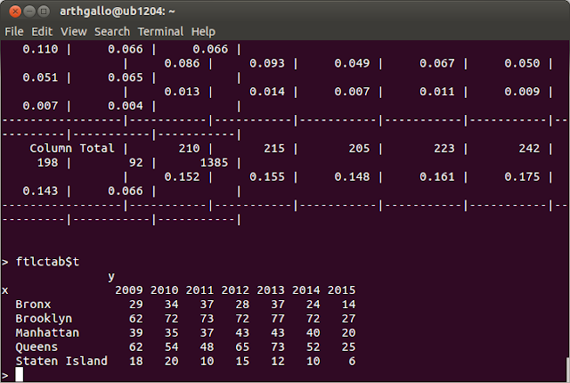
Next we will use the CrossTable function to look at number of accidents that involved one or more fatalities
We can instead also build a table to summarize fatalities by borough and year.
#Build a cross table for Borough name and Year with count of fatal incidents
ftlctab<-CrossTable(ftlty.f$BoroName,ftlty.f$YR,expected=FALSE)
ftlctab$t
 We can also build a cross table to look at number of fatalities using the xtabs function.
#Build a cross table for Borough name and Year with fatalities
ftlctab2<-xtabs(ftlty.f$Fatalities ~  ftlty.f$BoroName+ftlty.f$YR,ftlty.f)
ftlctab2
We can actually compare the results in the output above to see the differences.
We can also plot the above in barplots using the barplot command.
#Plot this on a barplot to see the trends for Incidents with fatalities
barplot(ftlctab$t
 ,col=c("red","orange","yellow","green","blue", "darkblue","grey")
 ,names.arg=levels(ftlty.f$YR)
 ,legend=rownames(ftlty.f$BoroName)
)
Now we could also plot the sum of fatalities instead of fatal incidents by using the ftlctab2 variable instead.
#Plot this on a barplot to see the trends for Fatalities
barplot(ftlctab2
 ,col=c("red","orange","yellow","green","blue", "darkblue","grey")
 ,names.arg=levels(ftlty.f$YR)
 ,legend=levels(ftlty.f$BoroName)
)
That's it. Here is the complete source code
# Load required libraries
library(rgdal)
library(ggplot2)
library(ggmap)
library(rgeos)
library(maptools)
library(scales)
library(gmodels)

# Set default paths for data
setwd("~/Work/Transportation/NYC/scripts")
shpfilepath="../data/shpfiles"

# Read injury and fatality statistics
ogrInfo(shpfilepath,"fatality_yearly")
ogrInfo(shpfilepath,"injury_yearly")
ftlty_yr<-readOGR(shpfilepath, "fatality_yearly")
injry_yr<-readOGR(shpfilepath, "injury_yearly")
names(ftlty_yr); dim(ftlty_yr)
names(injry_yr); dim(injry_yr)

# Add the spatial data to the data frame
ftlty.f <-fortify(as.data.frame(ftlty_yr))
names(ftlty.f);dim(ftlty.f)

#Load boroughs data
ogrInfo(shpfilepath,"nybbwi")
bbnd <- readOGR(shpfilepath,"nybbwi")

#Transform the coordinates from Lambert Conformal to Lat Long
CRS.latlong<-CRS("+proj=longlat +datum=WGS84 +no_defs")
bbnd<-spTransform(bbnd, CRS.latlong)

# Add the spatial data back to the boundary data.frame
bbnd.f <-fortify(bbnd, region="BoroCode")
names(bbnd.f);head(bbnd.f);dim(bbnd.f)

# Combine the geometry and data back together using common keys
bbnd.f<-merge(bbnd.f,bbnd@data, by.x="id", by.y="BoroCode")
names(bbnd.f);head(bbnd.f);dim(bbnd.f)

#Code each record in fatality with the borough it falls under and add to new variable
ftlty.f$BoroCode <-as.data.frame(over(ftlty_yr, bbnd))$BoroCode
ftlty.f$BoroName <-as.data.frame(over(ftlty_yr, bbnd))$BoroName
names(ftlty.f);head(ftlty.f);dim(ftlty.f)

#Plot accidents coded by the borough they fall in
fx<-ftlty.f$coords.x1
fy<-ftlty.f$coords.x2
Map <- ggplot(data=ftlty.f, aes(fx,fy,colour=factor(BoroCode)))
Map <- Map + layer(geom="point")
Map

#Build a cross table for Borough name and Year with count of fatal incidents
ftlctab<-CrossTable(ftlty.f$BoroName,ftlty.f$YR,expected=FALSE)
ftlctab$t

#Build a cross table for Borough name and Year with fatalities
ftlctab2<-xtabs(ftlty.f$Fatalities ~  ftlty.f$BoroName+ftlty.f$YR,ftlty.f)
ftlctab2

#Plot this on a barplot to see the trends for Incidents with fatalities
barplot(ftlctab$t
 ,col=c("red","orange","yellow","green","blue", "darkblue","grey")
 ,names.arg=levels(ftlty.f$YR)
 ,legend=rownames(ftlty.f$BoroName)
)

#Plot this on a barplot to see the trends for Fatalities
barplot(ftlctab2
 ,col=c("red","orange","yellow","green","blue", "darkblue","grey")
 ,names.arg=levels(ftlty.f$YR)
 ,legend=levels(ftlty.f$BoroName)
)


No comments:
Post a Comment