Plotting R data on an Interactive Google map

In this post, we will see how to plot data on an interactive map using R. We will use Google maps as the base map. Here is the output

You can also switch to street view

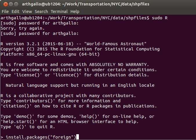
Let's get started. Make sure you have installed the required libraries. The new library needed is googleVis which can be installed by launching R in sudo mode and entering the following command

install.packages("googleVis")
q()

First step is to download the data. This previous post shows how to obtain the spatial data used in this example from the NYC website. Now launch R in regular mode and enter the following code to create the map.

First we need to load the required libraries

# Load the needed libraries
library(sp)  # classes for spatial data
library(maptools)
library(rgeos) # and their dependencies
library(rgdal)
library(ggplot2)
library(ggmap)
library(scales)
library(gmodels)
library(googleVis)

Next we need to set the working directory where our scripts are located and declare a variable to folder where our data is located.

# Set default paths for data
setwd("~/Work/Transportation/NYC/scripts")
shpfilepath="../data/shpfiles"

Next we will read the shape files with data. We have two shape files from NYC. First contains only fatal accidents, and second contains injury accidents. We will later combine these files.

# Read injury and fatality statistics
ogrInfo(shpfilepath,"fatality_yearly")
ogrInfo(shpfilepath,"injury_yearly")
ftlty<-readOGR(shpfilepath, "fatality_yearly")
injry<-readOGR(shpfilepath, "injury_yearly")
names(ftlty); dim(ftlty)
names(injry); dim(injry)

Next we need to rename the column names across the two datasets so that they are identical. Following step shows us how to do that. We also will add a new variable that classifies the incident as an injury or a fatality incident.

#Classify severity and rename columns to be identical in fatalities and injury datasets
ftlty$Severity<-"Fatality"
names(ftlty)[names(ftlty)=="Fatalities"]<-"Total"
names(ftlty)[names(ftlty)=="PedFatalit"]<-"Ped"
names(ftlty)[names(ftlty)=="BikeFatali"]<-"Bike"
names(ftlty)[names(ftlty)=="MVOFatalit"]<-"MVO"
injry$Severity<-"Injury"
names(injry)[names(injry)=="Injuries"]<-"Total"
names(injry)[names(injry)=="PedInjurie"]<-"Ped"
names(injry)[names(injry)=="BikeInjuri"]<-"Bike"
names(injry)[names(injry)=="MVOInjurie"]<-"MVO"
names(injry);names(ftlty)

Now we can combine the two datasets to create one single dataset called acc.

#Combine datasets
acc<- rbind(ftlty, injry)
dim(acc);names(acc);head(acc)

We need to use the fortify command to make sure the coordinate information can be accessed by spatial functions.

#Now fortify the accident data
acc.f<-fortify(as.data.frame(acc))
dim(acc.f);names(acc.f);head(acc.f)

We only want to plot 2015 data. The following command shows us how to filter only 2015 records from the data.

#Subsetting only 2015 accident records
acc_2015<-acc.f[which(acc.f$YR==2015),] 

Now we are ready to plot this on the map. The gvisMap function expects a single field with latitude and longitude information in lat:long format, that is separated by a colon. We don't need more than 4 digit precision so we will round the lat long information and use the paste command to concatenate everything into a single string.

#Add a single column "LatLong" that is of the format lat:long for the accident location
acc_2015$LatLong<-paste(round(acc_2015$coords.x2,4),round(acc_2015$coords.x1,4),sep=":")

The gVisMap function also expects a data field which will be displayed as a map tip. We need to concatenate all available fields with html break symbol to create one single field that can pop up when we hover or click on the icon.

#Add a single column "Tip" for Accident descriptions separated by html breaks ("<br/>")
acc_2015$Tip<-paste("Type: ",acc_2015$Severity,"Total: ",acc_2015$Total,"Ped: ",acc_2015$Ped,"Bike: ",acc_2015$Bike,"MVO: ",acc_2015$MVO,sep="<br/>")
head(acc_2015)

Finally, we call the gVisMap function passing the dataset, name of concatenated lat long column, name of the Map tip column and set several defaults for the Google map. Calling the plot function launches an embedded http server and launches the default browser on your machine to display the generated html page.

#Plot 2015 accidents on Google
map1<-gvisMap(acc_2015, "LatLong", "Tip", 
              options=list(showTip=TRUE, showLine=F, enableScrollWheel=TRUE, 
                           mapType='roads', useMapTypeControl=TRUE, width=800,height=1024))
plot(map1)

That's it... We are done. Here is the output

Here is the complete source code

# Load the needed libraries
library(sp)  # classes for spatial data
library(maptools)
library(rgeos) # and their dependencies
library(rgdal)
library(ggplot2)
library(ggmap)
library(scales)
library(gmodels)
library(googleVis)

# Set default paths for data
setwd("~/Work/Transportation/NYC/scripts")
shpfilepath="../data/shpfiles"

# Read injury and fatality statistics
ogrInfo(shpfilepath,"fatality_yearly")
ogrInfo(shpfilepath,"injury_yearly")
ftlty<-readOGR(shpfilepath, "fatality_yearly")
injry<-readOGR(shpfilepath, "injury_yearly")
names(ftlty); dim(ftlty)
names(injry); dim(injry)

#Classify severity and rename columns to be identical in fatalities and injury datasets
ftlty$Severity<-"Fatality"
names(ftlty)[names(ftlty)=="Fatalities"]<-"Total"
names(ftlty)[names(ftlty)=="PedFatalit"]<-"Ped"
names(ftlty)[names(ftlty)=="BikeFatali"]<-"Bike"
names(ftlty)[names(ftlty)=="MVOFatalit"]<-"MVO"
injry$Severity<-"Injury"
names(injry)[names(injry)=="Injuries"]<-"Total"
names(injry)[names(injry)=="PedInjurie"]<-"Ped"
names(injry)[names(injry)=="BikeInjuri"]<-"Bike"
names(injry)[names(injry)=="MVOInjurie"]<-"MVO"
names(injry);names(ftlty)

#Combine datasets
acc<- rbind(ftlty, injry)
dim(acc);names(acc);head(acc)

#Now fortify the accident data
acc.f<-fortify(as.data.frame(acc))
dim(acc.f);names(acc.f);head(acc.f)

#Subsetting only 2015 accident records
acc_2015<-acc.f[which(acc.f$YR==2015),] 

#Add a single column "LatLong" that is of the format lat:long for the accident location
acc_2015$LatLong<-paste(round(acc_2015$coords.x2,4),round(acc_2015$coords.x1,4),sep=":")

#Add a single column "Tip" for Accident descriptions separated by html breaks ("<br/>")
acc_2015$Tip<-paste("Type: ",acc_2015$Severity,"Total: ",acc_2015$Total,"Ped: ",acc_2015$Ped,"Bike: ",acc_2015$Bike,"MVO: ",acc_2015$MVO,sep="<br/>")
head(acc_2015)

#Plot 2015 accidents on Google
map1<-gvisMap(acc_2015, "LatLong", "Tip", 
              options=list(showTip=TRUE, showLine=F, enableScrollWheel=TRUE, 
                           mapType='roads', useMapTypeControl=TRUE, width=800,height=1024))
plot(map1)

Installing gmodels library in R

Steps for installing gmodels in your R distribution are fairly straight forward.

First login to R using sudo, so your package can be installed to the shared repository

sudo R

Next, enter the following command in R prompt

install.packages("gmodels")

By default, R prompts for https mirrors. For some reason, https mirrors gave me errors. For this reason select the option for HTTP mirrors at the bottom of the list, as shown below.

Next, choose your preferred mirror from the list of http mirrors, as shown below

Click OK to install. R will download the packages and install as neccessary.

Once the installation, has finished load the library using the following command and we are good to go.

library(gmodels)

That's it...

Reading shape files in R

In the previous post, we saw how to read dbf files in R. I wanted to go a step further.

I was looking at ways to read shape file data in R. It turns out there are various mechanisms for doing just that. However, for the library to be installed correctly, your environment needs to be setup correctly.

Here are the steps I followed.

1. Install libgdal
2. Install libproj
3. Install rgdal package
4. Test loading a shape file

The following script should install these packages correctly for you.

sudo apt-get install apt-file
sudo apt-get update
sudo apt-get install libgdal1h
sudo apt-get install libgdal1-dev libproj-dev

Once these packages are setup correctly start R as sudo

sudo R

Enter the following commands on the R console

install.packages("rgdal")
install.packages("rgeos")
install.packages("ggmap")
install.packages("maptools")
q()

The following screen shows installation for rgeos

Next run the following commands in R (without sudo)

library(rgdal)
shpfilepath="../data/shpfiles"
ogrInfo(shpfilepath,"fatality_yearly")
ftlty_yr <-readOGR(shpfilepath, "fatality_yearly")

This shows the following:

Now, enter the following command in R

plot(ftlty_yr, axes=TRUE, border="gray")

Our R environment can now read shapefiles correctly

Reading dbf files in R

In this post, we will see how to load dbf tables in R.

First item is to install the appropriate R library. In this case, it happens to be a library called foreign.

Run R in administrative mode so that library can be installed in the universal library

sudo R

> install.packages("foreign")

Quit R and re-enter R in non-administrative (non-sudo) mode

At, the R prompt, enter the following commands

 library(foreign)  
 fatal_yr <- read.dbf("~/Work/Transportation/NYC/data/shpfiles/fatality_yearly.dbf")  
 dim(fatal_yr)  

That's it, we have loaded the dbf file.

Generating Poisson Distributed time events with R

In this example, I would like to generate a set of values that is based on a set of discrete arrivals. Poisson distribution is ideal for generating these random values. Lets say I want to generate a set of time events for cars arriving into an on-street parking next to a strip mall at a rate of average 2 to 3 per minute. Maximum arrivals are at 9:00 am. Total number of parking available is 10. If parking is available, a car parks for a mean of 45 minutes. If not, drivers look for additional parking around.

To start with, we can start arrivals at 6 AM till 10:00 PM. That is 16 hours. Also, let us assume an average of 3 cars per minute. To make sure, we can generate sub-minute arrivals, we need to convert everything to seconds. In this first attempt, we will ignore that arrival rate is time dependent and assume a homogeneous arrival rate through out the day. We will tackle inhomogeneous time-dependent arrival rates in a future post.

To generate these numbers, we can use the following formula

rate <- 3/60

period <- 16*60*60

start <- 6*60*60

cars <- runif(rpois(1,period*rate), min=start, max=start+period)

To see, how the data is distributed over time, we can see the individual arrivals per hour as a histogram with the following command.

> hist(cars, breaks=16)

To see arrivals per minute, we can use the following command.

> hist(cars, breaks=16*4)

To see the actual data generated, we can just type cars on the prompt to see the generated vector.

We will carry on from here...